A Quick Review
Happy Super Bowl Sunday! In my last post, I illustrated how to write a function for fitting logistic regression, a common model for classifying dichotomous categorical outcomes. The model predicted the probability that y equaled class 1 (\(p(y = 1|X)\)) by applying a sigmoid transformation to the linear combination of predictors(\(\frac{1}{(1+e^{-(X\beta)})}\)). Regression weights were chosen such that the likelihood of the observed data given beta (\(p(y|\beta)\)) was maximized.
What can be improved on?
Our maximum likelihood implementation is nice, but it has some significant shortcomings “as is”. First, traditional maximum likelihood logistic regression does not take into account prior information. Ignoring prior information makes it difficult to refit the model as new batches of data come in. Consider the motivating example from the previous post. Our goal was to build a classification system to predict the probability of an employee accepting a job offer. As hiring cycles begin and end, users may want to update their model with each new batch of data that comes in! Our function as is, cannot accommodate updates and must be refit using all available data. Storing this amount of data can lead to extensive (and unnecessary) database management costs. While this may not be a big deal for small organizations, when working with large organizations this could become a sizable cost! It would be nice if we could simply store some aspects of the model and then update our model as new information comes in.
Not only do traditional maximum likelihood estimates fail to account for prior information, it approaches uncertainty in parameter estimates in a rather unrefined way. Maximum likelihood is rooted in frequentest notions of probability. In short, frequentists approach probability as the expected value of a series of infinite repeated trials. In other words, frequentists make the assumption that there is some true parameter \(\theta\), that generates the observed data. They use the expected values of the theta (often estimated through maximum likelihood) to make their best guess about the “true parameter”. In some cases this is an extremely useful approach to probability! In others, such as one off or rare events where repeated trials are not possible, this interpretation doesn’t map to reality.
This approach to probability makes explaining some aspects of frequentist statistics sometimes difficult. For example, frequentists quantify their uncertainty about parameter estimates using confidence intervals which have a rather unnatural interpretation. These intervals can only be interpreted in terms of repeated trials. Imagine I were to quantify uncertainty in an estimate of the expected number of heads in a set of 10 coin tosses (CI95% = [3, 7]). This interval cannot be interpreted as the range of values that we are 95% certain the true average number of heads falls in. This range can only be interpreted in the context of repeated experiments and calculations of confidence intervals. In other words, a 95% CI is the range of values that, if the experiment were repeated and CIs were calculated a large number of times (say 1000), would contain the true mean 95% of the time.
What does a Bayesian perspective contribute?
The Bayesian perspective addresses both of these short comings by defining and estimating a full probability model. Some may recognize the below formula as Bayes rule.
\[p(A|B) = \frac{p(B|A)p(A)}{p(B)}\]
Let’s put things in terms of our logistic regression model. We have a set of parameters, \(\beta\), our data, \(D\), and a set of prior beliefs about beta \(\beta_{prior}\). We are interested in describing the density of \(p(\beta|D)\), which is often referred to as the posterior distribution. However, the maximum likelihood approach we implemented previously focuses exclusively on \(p(D|\beta)\). We can implement Bayes rule in this scenario by modeling:
\[p(\beta|D) = \frac{p(D|\beta)p(\beta|\beta_{prior})}{p(D)}\]
Lucky for us there are some familiar terms! We know that the likelihood formula above is equivalent to the \(p(D|\beta)\). The term \(p(\beta|\beta_{prior})\) is simply a probability density or the prior evaluated at \(\beta\). For example, if we use a normal prior on the regression coefficients, \(p(\beta|\beta_{prior})\) could be solved for using dmvnorm(beta, mu_beta_prior, Sigma_beta_prior). Plugging in the likelihood for \(P(D|\beta)\) and using our new understanding of \(P(\beta|\beta_{prior})\) we are left with \(p(D)\).
\[p(\beta|D) = \frac{L(\beta)p(\beta|\beta_{prior})}{p(D)}\]
\(p(D)\) is a scaling constant that ensures the product of the likelihood an prior terms integrate to 1. Unfortunately in our case there is no analytic solution for \(P(D)\). This is because when we apply the sigmoid transformation to the linear model, we remove the possibility of finding conjugate priors (see here). Instead of using formulaic methods we must rely on true Bayesian methods that simulate the posterior distribution (Hamiltonian Markov Chain Monte Carlo) or approximate the posterior.
So what does this new approach buy us? Well, for starters, we can account for prior information. Furthermore, the posteriors of the model can often be summarized by distributional parameters making the storage requirements for the model very small. Iteratively updating priors and posteriors as new information comes in allows our algorithms to learn and update over time. Finally, by conditioning \(\beta\) on prior information, we can actually talk about probability in terms that are much easier to explain to stakeholders. For example, the 5th and 95th percentiles of the posterior can directly be interpreted as the range of values for which we are 95% certain the “true” parameter lies (assuming you are willing to accept there is a “true” parameter).
Markov Chain Monte Carlo
Given that there is no closed form solution for the posterior of logistic regression, how can we capitalize on the benefits of Bayesian regression? Markov Chain Monte Carlos are a class of methods used to simulate the posterior distribution of a set of parameters \(\theta\). The intuition behind them is relatively simple. In cases where there is not an easy way to calculate a normalizing constant, we can iteratively simulate draws from the distribution of \(\theta\).
To simulate these draws, we first pick a starting value for our algorithm. Next, we propose a new value of theta by adding a random number to the start point. If that value is more likely than the starting point, given the data we observed and our priors, we accept this new theta and store it as a possible value. If the new theta’s likelihood is less than the starting point we (probably) reject this as being a possible value of theta. We then add another random number to the most recent accepted theta and repeat the process. After thousands of iterations we can look at the distribution of theta and get a good idea at the distribution of possible values for our parameters of interest. I include quasi-code down below to better illustrate the algorithm I just described. This is, in fact, the Metropolis algorithm and gives a good intuition about the purpose of more advanced Markov Chain Monte Carlo methods.
Metropolis Algorithm
Define y, X, prior_theta, theta_start, maxit;

Initialize theta = theta_start;
Initialize p_theta = p(y | theta_start) * p(theta_start | prior_theta);
Initialize counter = 1;
Initialize post_dist = vector(mode = "numeric");

for t in 1 to maxit;

  proposal = theta + rnorm(1);

  p_proposal = p(y | proposal) * p(proposal | prior_theta)

  ratio = p_propoal / p_theta;

  if ratio >= 1;
    accept_proposal = TRUE;
  else;
    accept_proposal = as.logical(rbinom(n = 1, size = 1, prob = ratio));
  end;

  if accept_proposal = TRUE;
    theta =  proposal;
    p_theta = p_proposal;
    post_dist[counter] = theta;
    counter += 1;
  end;
end;

return post_dist;
While I do love creating algorithms from scratch, creating an efficient Markov Chain Monte Carlo function that works in a variety of cases ends up being a TON of work. The issues stems from the jump distribution (the distribution from which proposal thetas are selected). Sadly, for this chapter, I am going to rely on the brms package to get the job done. I say “sadly”, but brms is a fantastic package that I would recommend to anyone! For those of you who like developing from scratch algorithms, I will show a speedy alternative to MCMC in the section that follows.
I am going to be working with a similar data frame as the last post, although I am cutting down the size in order to decrease the models’ run times. MCMC is pretty slow furthermore I want to illustrate how Bayesian learning can be implemented. To further facilitate this process and clean up the code I define a few helper functions below. These aren’t generalizable but do clean up the code.
# Simulation Parameters
fe<-c("Intercept" = 0, "salary" = .3, "job_alt" = 1, "flexibility" = .3, "difficulty"  = -2, "market_sal" = -.15)
# Helper functions for summarising the posterior distribution
post_summary<-function(model){
model%>%
spread_draws(b_Intercept, b_salary, b_job_alt, b_difficulty, b_flexibility, b_market_sal)%>%
select(b_Intercept:b_market_sal)%>%
rename_all(.funs = ~str_remove(., "^b_"))%>%
gather(key = var, value = value)%>%
group_by(var)%>%
summarise(mean = mean(value),
sd = sd(value),
p_95 = quantile(value, .95),
p_05 = quantile(value, .05))
}
# Defining Helper function to iteratively update priors using posterior summary tables
prep_priors<-function(post_summary){
# Creating necessary dataframe for brms prior construction
prior_df<-post_summary%>%
transmute(prior = paste0("normal(", mean, ",", sd, ")"),
class = if_else(str_detect(var, "Intercept"), "Intercept", "b"),
coef = if_else(str_detect(var, "Intercept"), "", str_remove(var, "^b_")))
# applying beta_df
beta_df<-prior_df%>%
filter(class != "Intercept")
intercept_df<-prior_df%>%
filter(class == "Intercept")
new_priors<-empty_prior()
for(i in 1:nrow(beta_df)){
new_priors[i,]<- prior_string(beta_df$prior[i], class = beta_df$class[i], coef = beta_df$coef[i])
}
new_priors[nrow(prior_df),]<- prior_string(intercept_df$prior[1], class = intercept_df$class[1])
new_priors
}
# Linear combination of predictors
v<-function(X, beta){
v<-X%*%beta
v
}
# Estimated Probability through sigmoid transformation
p_hat<-function(v){
p<-1/(1+exp(-v))
p
}Let’s begin the model building process by defining our priors. In our problem set up, we are implementing a new system so for now we will apply a diffuse prior on each coefficient. For the sake of simplicity (and capitalizing because of the central limit theorem), I am assuming that the intercept and regression weights are normally distributed. Kind of a cool side note, this prior specification is actually identical to ridge regression and acts as a regularization method.
library(brms)
library(tidybayes)
library(gganimate)

# Setting Priors
m1priors <- c(
  prior(normal(0,3), class = "Intercept"),
  prior(normal(0,3), class = "b", coef = "flexibility"),
  prior(normal(0,3), class = "b", coef = "job_alt"),
  prior(normal(0,3), class = "b", coef = "salary"),
  prior(normal(0,3), class = "b", coef = "difficulty"),
  prior(normal(0,3), class = "b", coef = "market_sal")
)
The model results are interesting and depict quite a bit of uncertainty in our estimates. In fact, the plausible values for theta are in some cases quite wide
# Running model
m1 <- brms::brm(
  decision ~ salary+job_alt+difficulty+flexibility+market_sal,
  data = dec,
  prior = m1priors,
  family = "bernoulli",
  seed = 123 # Adding a seed makes results reproducible.
)
# Printing output
summary(m1)## Family: bernoulli
## Links: mu = logit
## Formula: decision ~ salary + job_alt + difficulty + flexibility + market_sal
## Data: dec (Number of observations: 50)
## Samples: 4 chains, each with iter = 2000; warmup = 1000; thin = 1;
## total post-warmup samples = 4000
##
## Population-Level Effects:
## Estimate Est.Error l-95% CI u-95% CI Rhat Bulk_ESS Tail_ESS
## Intercept 0.21 3.89 -7.99 7.14 1.00 3395 2984
## salary 0.93 0.39 0.29 1.84 1.00 1823 1859
## job_alt 2.30 0.89 0.68 4.18 1.00 1710 2031
## difficulty -4.99 1.44 -8.17 -2.54 1.00 1608 2174
## flexibility 2.07 1.08 0.32 4.49 1.00 2564 2428
## market_sal -0.57 0.25 -1.11 -0.14 1.00 1863 2363
##
## Samples were drawn using sampling(NUTS). For each parameter, Eff.Sample
## is a crude measure of effective sample size, and Rhat is the potential
## scale reduction factor on split chains (at convergence, Rhat = 1).post<-post_summary(m1)
# Plotting Posterior Estimates
post%>%
ggplot(aes(x = var, y = mean))+
geom_bar(stat = "identity")+
geom_errorbar(aes(ymin = p_05,
ymax = p_95),
width = .3)+
geom_point(data = fe_data, aes(x = var, y = value))+
labs(x = "", y = "Estimate",
title = "Posterior Estimates of Logistic Regression Coefficients",
subtitle = "Points represent simulation parameters.")+
theme(panel.grid = element_blank())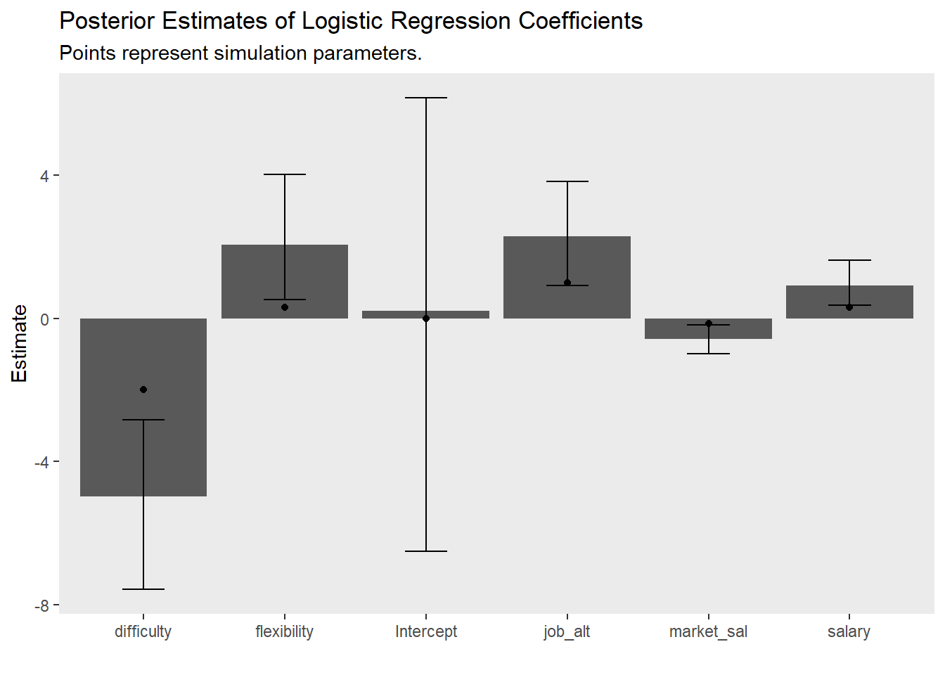
Below I implement an iterative update procedure over 10 data collection points to illustrate how Bayesian learning can be beneficial. In short this simulates how Bayesian models can be updated as new information comes in. After each iteration, I save the mean posterior estimate and use that as the prior for the next wave of data. I also calculate the average cost my model incurs at each time point, which is given by the mean absolute difference between the predicted and observed outcome. This provides an indication of how well the model is learning. If the cost is decreasing as time increases, the model is learning As a references, I plot the batch approach which uses all available data to make predictions about future observations.
##### Bayesian Approach ######
# Initializing parameters -----------------------------------------------------------------------
# Initalizing priors for first time point
# This initializes the same priors as above for =but formats them so they can be updated in the loop
post<-data.frame(var = paste0("b_", post$var),
                 mean = rep(0, length(post$var)),
                 sd = rep(3, length(post$var)))

# initialized relevant objects for manipulation and storage
f<-decision ~ salary+job_alt+difficulty+flexibility+market_sal
y_name<-"decision"
regret<-c()
post_list<-list()

## Beginning for loop
for (j in 1:10){

# Solving for regret ---------------------------------------------------------------------------
  X<-model.matrix(f, data_list[[j]])
  y<-data_list[[j]][y_name]%>%
    as.matrix()%>%
    as.vector()

  beta<-as.matrix(post$mean)[c(3, 6, 4, 1, 2, 5),]
  v_hat<-v(X, beta)
  p<-p_hat(v_hat)

 regret[j]<- mean(abs(y-p))


# Set Priors -----------------------------------------------------------------------------------
new_priors<-prep_priors(post)

# Run model
new_model <- brms::brm(
  f,
  data = data_list[[j]],
  prior = new_priors,
  family = "bernoulli",
  seed = 123 # Adding a seed makes results reproducible.
)

  post<-post_summary(new_model)

  post_list[[j]]<-post
}
##### Frequentist Approach ######
regret_freq<-c()
model_list<-list()
for (j in 1:10){
y<-data_list[[j]][y_name]%>%
as.matrix()%>%
as.vector()
if(j == 1){
regret_freq[j]<-mean(abs(y-.5))
}else{
regret_freq[j]<-mean(abs(y-predict(freq_model, newdata = data_list[[j]], type = "response")))
}
# Run model
freq_model <- glm(
f,
data = bind_rows(data_list[1:j]),
family = "binomial",
)
model_list[[j]]<-freq_model
}## Warning: glm.fit: fitted probabilities numerically 0 or 1 occurredpost_df<-map_dfr(1:length(post_list), function(x){
post_list[[x]]%>%mutate(iteration = x)
})post_df%>%
ggplot(aes(x = var, y = mean))+
geom_bar(stat = "identity")+
geom_errorbar(aes(ymin = p_05,
ymax = p_95),
width = .3)+
geom_point(data = fe_data, aes(x = var, y = value))+
labs(x = "", y = "Estimate",
title = "Posterior Estimates of Logistic Regression Coefficients at Time {closest_state} of 10",
subtitle = "Points represent simulation parameters.")+
theme(panel.grid = element_blank())+
transition_states(iteration,
transition_length = 2,
state_length = 1)
tibble(`Update Method` = rep(c("Bayesian", "Batch"), each = 10),
           time = rep(1:10, times = 2),
           cost = c(regret, regret_freq))%>%
  ggplot(aes(x = time, y = cost, lty = `Update Method`))+
  geom_line()+
  labs(x = "Time", y = "Cost",
       title = "Cost Incurred at Time t")+
  theme(panel.grid = element_blank())+
 scale_x_continuous(breaks = 1:10)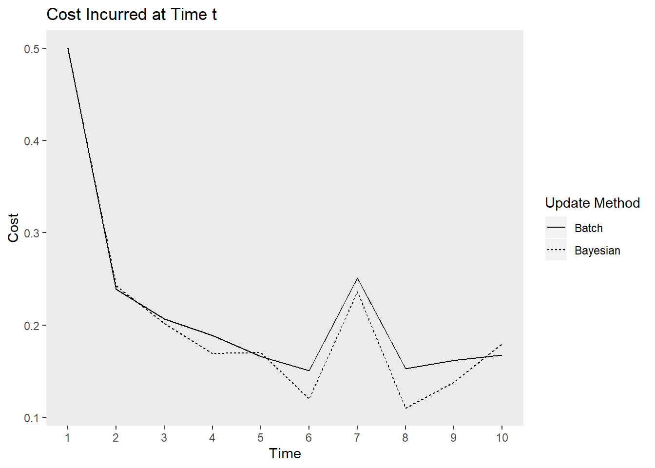
Laplace Approximation
While MCMC is super flexible, it isn’t the most scalable solution. This is because it is rather slow - especially implemented through brms which requires the compilation of a c++ model. The primary problem with Bayesian logistic regression is that the we can’t solve analytically for \(p(D)\). A work around is to solve for the mean a posteriori given normal priors and than approximate the distribution with a Taylor expansion (covered here in the context of optimization) about the estimate.
How do we solve for the mean a posteriori estimate? This is done my maximizing the joint likelihood:
\[p(D|\beta)p(\beta|\beta_{prior})\]
\(P(D|\beta)\) is simply the typical likelihood for binomial random variables.
\[L(\beta) = -\sum_{i=1}^n\ y_i\ ln(\ \hat p_i(y = 1)\ )+(1-y_i)\ ln(\ 1-\hat p_i(y = 1)\ )\] \(p(\beta|\beta_{prior})\) can be solved simply using the multivariate normal density. This means that in order to solve for the mean a posteriori we need to
\[\min_\theta -(\sum_{i=1}^n\ y_i\ ln(\ \hat p_i(y = 1)\ )+(1-y_i)\ ln(\ 1-\hat p_i(y = 1)\ ))+log((\theta-\mu)\Sigma^{-1}(\theta-\mu)))\]
# Defining Objective Function ----------------------------------------------------------------
post_ll<-function(theta, X, y, prior_beta, prior_vcov){

  v_hat<-v(X = X, beta = theta)
  p<-p_hat(v_hat)

  ll_x<--sum(y*log(p)+(1-y)*log(1-p))
  ll_p<--log(mixtools::dmvnorm(y = theta-prior_beta, mu = rep(0, length(theta)), sigma = prior_vcov))

  ll_post<- ll_x+ll_p

  ll_post
}
The Taylor expansion has some cool properties. First, by minimizing the joint likelihood with respect to theta, we set the first derivative equal to 0. This means that the first order term drops out leaving the Taylor expansion with only the inverse hessian. Since derivatives are additive we can chunk the objective function to solve for the hessian. The first part of the equation is composed of the typical likelihood function for a binomial random variable. We solved for the hessian in the first post. The second part is the multivariate normal density which has a well known hessian (\(\Sigma^{-1}\)). We can simply add the covariance matrix of the priors to the hessian of the likelihood to solve for the Taylor expansion.
# Implementation of Laplace ----------------------------------------------------------------
logistic_laplace<-function(formula=NULL, data=NULL, prior_beta=NULL, prior_vcov=NULL, X, y){

  # Prepping requisite objects -----------------------------------------------------------
  if(!is.null(formula) & !is.null(data)){
    X<-model.matrix(formula, data)
    y<-as.vector(as.matrix(data[as.character(formula)[2]]))
  }

  p<-ncol(X)

  # Handling priors if non are provided ---------------------------------------------------
  if(is.null(prior_beta)){
    prior_beta<-rep(0, p)
  }

  if(is.null(prior_vcov)){
    prior_vcov<-diag(5, nrow = p, ncol= p)
  }

  # Solving for theta --------------------------------------------------------------------------
    # using optim is cheating, I know
    # Solution for the hessian is outlined above and the derivatives are pretty easy
    # I think the motivated person would be able to implement newtonian optimization without me spelling it out
   rs<-optim(par = prior_beta, post_ll, hessian = TRUE, prior_beta = prior_beta, prior_vcov = prior_vcov, X = X, y = y)

   post_beta<-rs$par

   post_cov<-solve(rs$hessian)

   list(MAP = post_beta,
        vcov = post_cov)
}

# Helper function for posterior extraction from lists-------------------------------------------

laplace_posterior<-function(model_list, coef_names){
  vcov_list<-map(model_list, "vcov")
  coef_list<-map(model_list, "MAP")


  vcov<-map_dfr(vcov_list, function(x){
                                   variance<- diag(x)
                                   names(variance)<-coef_names
                                   variance<-t(variance)
                                   as.data.frame(variance)}
          )%>%
  mutate(Time = 1:n())%>%
  gather(key = "Coefficient",
             value = "VAR",
             - Time)


map<-map_dfr(coef_list, function(x){names(x)<-coef_names
                                   x<-t(x)
                                   as.data.frame(x)}
        )%>%
      mutate(Time = 1:n())%>%
      gather(key = "Coefficient",
             value = "MAP",
             - Time)

posterior_dist<-left_join(map, vcov)

posterior_dist
}
When do Laplace approximations work? The Taylor expansion implies that the posterior distribution will me normal. They work well in scenarios for which a normal posterior would be appropriate. Given that a normal posterior is typically appropriate for GLM models when the sample size is sufficiently large, this is often a good candidate for the priors. Below, I am going to replicate the analysis done above, but then explore some slight variations that weren’t possible with brms because of run-time restrictions. In the first variation, I am going to update the models with smaller batches (but the same overall sample size n = 500). Second, I am going to explore how the model performs when the simulation parameters are not stationary.
Simulation 1: 50 Observation Batches with Deterministic Data Generation
This simulation is intended to replicate the analyses above. It provides insight into how much more cost our learner incurs relative to the batch method that requires full data storage and the MCMC approach which takes much longer. The gif below illustrates how quickly the model recovers the simulation parameters. The cost function is also plotted over time.
# Define initial priors
prior_beta<-rep(0, 6)
prior_vcov<-diag(3, 6)

# Initialize storage and useful objects
model_list<-list()
loss<-vector("numeric")

f<-decision~salary+job_alt+flexibility+difficulty+market_sal
y_name<-"decision"

for(i in 1:10){

  # Solving for the cost -----------------------------
    X<-model.matrix(f, data_list[[i]])
    y<-as.vector(as.matrix(data_list[[i]][y_name]))
    v_hat<-v(X, prior_beta)
    p<-p_hat(v_hat)
    loss[[i]]<-mean(abs(y-p))

  # Running model -------------------------------------
  m<-logistic_laplace(f,
                      data = data_list[[i]],
                      prior_beta = prior_beta,
                      prior_vcov = prior_vcov)

  # Updating Priors -----------------------------------
  prior_beta<-m$MAP
  prior_vcov<-m$vcov

  # Storing model output ------------------------------
  model_list[[i]]<-m
}

# Defining coefficient names
coef_names<-c("Intercept", "salary", "job_alt", "flexibility", "difficulty", "market_sal")

laplace_summary<-laplace_posterior(model_list = model_list, coef_names = coef_names)
## Joining, by = c("Time", "Coefficient")##### Frequentist Approach ######
regret_freq<-c()
model_list<-list()
for (j in 1:10){
y<-data_list[[j]][y_name]%>%
as.matrix()%>%
as.vector()
if(j == 1){
regret_freq[j]<-mean(abs(y-.5))
}else{
regret_freq[j]<-mean(abs(y-predict(freq_model, newdata = data_list[[j]], type = "response")))
}
# Run model
freq_model <- glm(
f,
data = bind_rows(data_list[1:j]),
family = "binomial",
)
model_list[[j]]<-freq_model
}laplace_summary%>%
ggplot(aes(x = Coefficient, y = MAP))+
geom_bar(stat = "identity")+
geom_errorbar(aes(ymin = MAP-2*sqrt(VAR),
ymax = MAP+2*sqrt(VAR)),
width = .3)+
geom_point(data = fe_data, aes(x = var, y = value))+
labs(x = "", y = "Estimate",
title = "Posterior Estimates of Logistic Regression Coefficients at Time {closest_state} of 10",
subtitle = "Points represent simulation parameters.")+
theme(panel.grid = element_blank())+
transition_states(Time,
transition_length = 2,
state_length = 1)
tibble(`Update Method` = rep(c("Laplace Approximation", "Batch"), each = 10),
           time = rep(1:10, times = 2),
           cost = c(loss, regret_freq))%>%
  ggplot(aes(x = time, y = cost, lty = `Update Method`))+
  geom_line()+
  labs(x = "Time", y = "Cost",
       title = "Average Cost Incurred at Time t")+
  theme(panel.grid = element_blank())+
 scale_x_continuous(breaks = 1:10)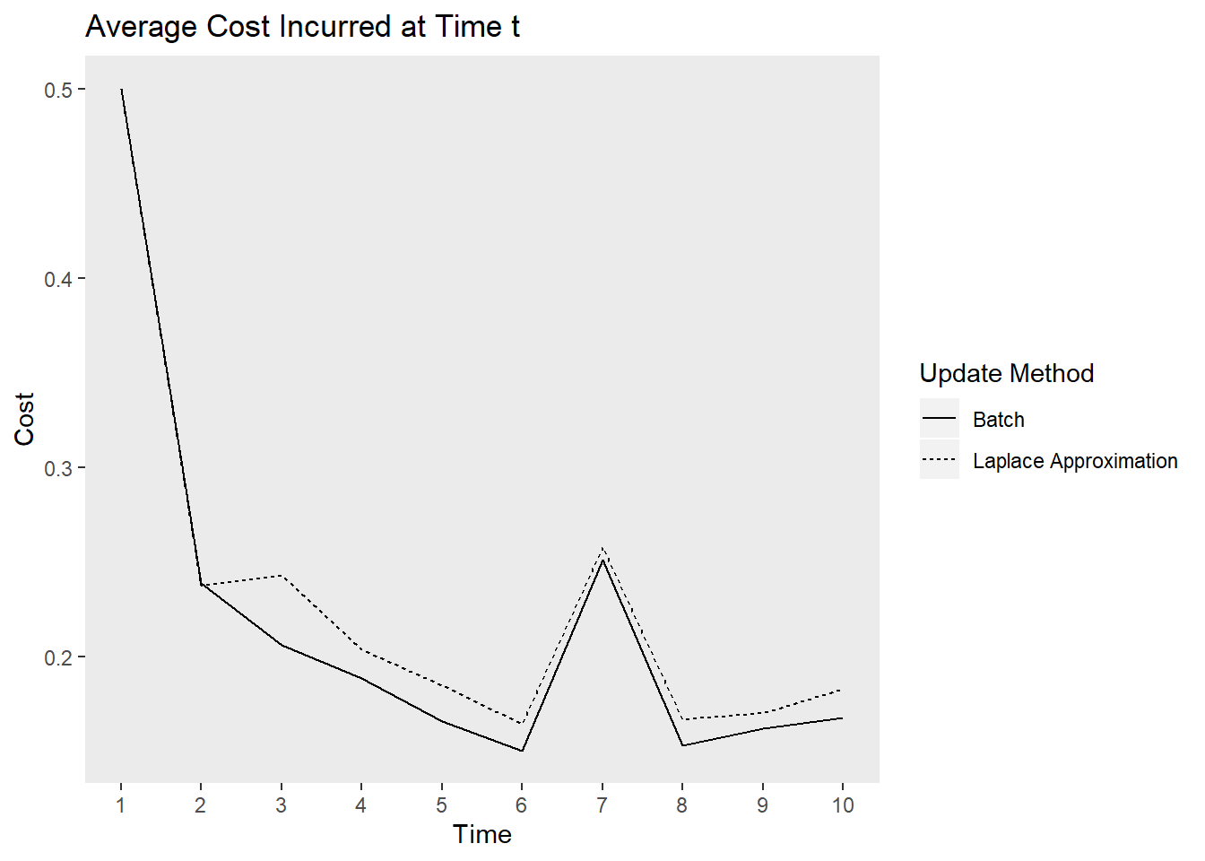
Simulation 2: 5 Observation Batches with Deterministic Data Generation
In some situations we may be interested in more frequent updates. This results in a noisier learning process but may make the model more quickly adjust to changes in the data generation process. In this case the data structure is deterministic, meaning that the data generation process is not changing. In this case, it doesn’t seem like we gain or lose much by this smaller batch size. With the exception of a small peak at the beginning the Laplace approximation seems to hone in to the asymptotic error rate pretty quick.
# Define initial priors
prior_beta<-rep(0, 6)
prior_vcov<-diag(3, 6)

# Initialize storage and useful objects
model_list<-list()
loss<-vector("numeric")

f<-decision~salary+job_alt+flexibility+difficulty+market_sal
y_name<-"decision"

for(i in 1:100){

  # Solving for the cost -----------------------------
    X<-model.matrix(f, data_list[[i]])
    y<-as.vector(as.matrix(data_list[[i]][y_name]))
    v_hat<-v(X, prior_beta)
    p<-p_hat(v_hat)
    loss[[i]]<-mean(abs(y-p))

  # Running model -------------------------------------
  m<-logistic_laplace(f,
                      data = data_list[[i]],
                      prior_beta = prior_beta,
                      prior_vcov = prior_vcov)

  # Updating Priors -----------------------------------
  prior_beta<-m$MAP
  prior_vcov<-m$vcov

  # Storing model output ------------------------------
  model_list[[i]]<-m
}


laplace_summary<-laplace_posterior(model_list = model_list, coef_names)
## Joining, by = c("Time", "Coefficient")##### Frequentist Approach ######
regret_freq<-c()
model_list<-list()
for (j in 1:100){
y<-data_list[[j]][y_name]%>%
as.matrix()%>%
as.vector()
if(j == 1){
regret_freq[j]<-mean(abs(y-.5))
}else{
regret_freq[j]<-mean(abs(y-predict(freq_model, newdata = data_list[[j]], type = "response")))
}
# Run model
freq_model <- glm(
f,
data = bind_rows(data_list[1:j]),
family = "binomial",
)
model_list[[j]]<-freq_model
}laplace_summary%>%
ggplot(aes(x = Coefficient, y = MAP))+
geom_bar(stat = "identity")+
geom_errorbar(aes(ymin = MAP-2*sqrt(VAR),
ymax = MAP+2*sqrt(VAR)),
width = .3)+
geom_point(data = fe_data, aes(x = var, y = value))+
labs(x = "", y = "Estimate",
title = "Posterior Estimates of Logistic Regression Coefficients at Time {closest_state} of 100",
subtitle = "Points represent simulation parameters.")+
theme(panel.grid = element_blank())+
transition_states(Time,
transition_length = 2,
state_length = 1)
tibble(`Update Method` = rep(c("Laplace Approximation", "Batch"), each = 100),
           time = rep(1:100, times = 2),
           cost = c(loss, regret_freq))%>%
  ggplot(aes(x = time, y = cost, lty = `Update Method`))+
  geom_line()+
  labs(x = "Time", y = "Cost",
       title = "Average Cost Incurred at Time t")+
  theme(panel.grid = element_blank(),
        axis.text.x = element_text(angle = 95, vjust = .5, hjust = 1))+
 scale_x_continuous(breaks = seq(0, 100, by = 5))
Simulation 3: 50 Observation Batches with Fluctuating Data Generation
The final question is how do these methods compare when the data generation process changes. I introduce a large random jump downward at time point 50, which is a rather extreme example! I also increased the batch size to 50 to provide the learners a better chance at recovering from the change. The Bayesian model recovers much quicker than the batch model as indicated by the cost plot. The learner still struggles to recover the parameters after the shift, perhaps because the model was relatively certain that the parameters were positive but after the shift they jumped downwards. The uncertainty of parameter estimates did not seem to increase as time went on, which I found interesting! It seems the priors are severely restricting the influence of the likelihood. Perhaps in an applied situation, practitioners would be able to recognize such a sizable shift in the labor market!
# Define initial priors
prior_beta<-rep(0, 6)
prior_vcov<-diag(3, 6)

# Initialize storage and useful objects
model_list<-list()
loss<-vector("numeric")

f<-decision~salary+job_alt+flexibility+difficulty+market_sal
y_name<-"decision"

for(i in 1:100){

  # Solving for the cost -----------------------------
    X<-model.matrix(f, data_list[[i]])
    y<-as.vector(as.matrix(data_list[[i]][y_name]))
    v_hat<-v(X, prior_beta)
    p<-p_hat(v_hat)
    loss[[i]]<-mean(abs(y-p))

  # Running model -------------------------------------
  m<-logistic_laplace(f,
                      data = data_list[[i]],
                      prior_beta = prior_beta,
                      prior_vcov = prior_vcov)

  # Updating Priors -----------------------------------
  prior_beta<-m$MAP
  prior_vcov<-m$vcov

  # Storing model output ------------------------------
  model_list[[i]]<-m
}

# Defining coefficient names
coef_names<-c("Intercept", "salary", "job_alt", "flexibility", "difficulty", "market_sal")


laplace_summary<-laplace_posterior(model_list = model_list, coef_names)
## Joining, by = c("Time", "Coefficient")##### Frequentist Approach ######
regret_freq<-c()
model_list<-list()
for (j in 1:100){
y<-data_list[[j]][y_name]%>%
as.matrix()%>%
as.vector()
if(j == 1){
regret_freq[j]<-mean(abs(y-.5))
}else{
regret_freq[j]<-mean(abs(y-predict(freq_model, newdata = data_list[[j]], type = "response")))
}
# Run model
freq_model <- glm(
f,
data = bind_rows(data_list[1:j]),
family = "binomial",
)
model_list[[j]]<-freq_model
}laplace_summary%>%
ggplot(aes(x = Coefficient, y = MAP))+
geom_bar(stat = "identity")+
geom_errorbar(aes(ymin = MAP-2*sqrt(VAR),
ymax = MAP+2*sqrt(VAR)),
width = .3)+
geom_point(data = non_stat, aes(x = var, y = value))+
labs(x = "", y = "Estimate",
title = "Posterior Estimates of Logistic Regression Coefficients at Time {closest_state} of 100",
subtitle = "Points represent simulation parameters.")+
theme(panel.grid = element_blank())+
transition_states(Time,
transition_length = 2,
state_length = 1)
tibble(`Update Method` = rep(c("Laplace Approximation", "Batch"), each = 100),
           time = rep(1:100, times = 2),
           cost = c(loss, regret_freq))%>%
  ggplot(aes(x = time, y = cost, lty = `Update Method`))+
  geom_line()+
  labs(x = "Time", y = "Cost",
       title = "Average Cost Incurred at Time t")+
  theme(panel.grid = element_blank(),
        axis.text.x = element_text(angle = 95, vjust = .5, hjust = 1))+
 scale_x_continuous(breaks = seq(0, 100, by = 5))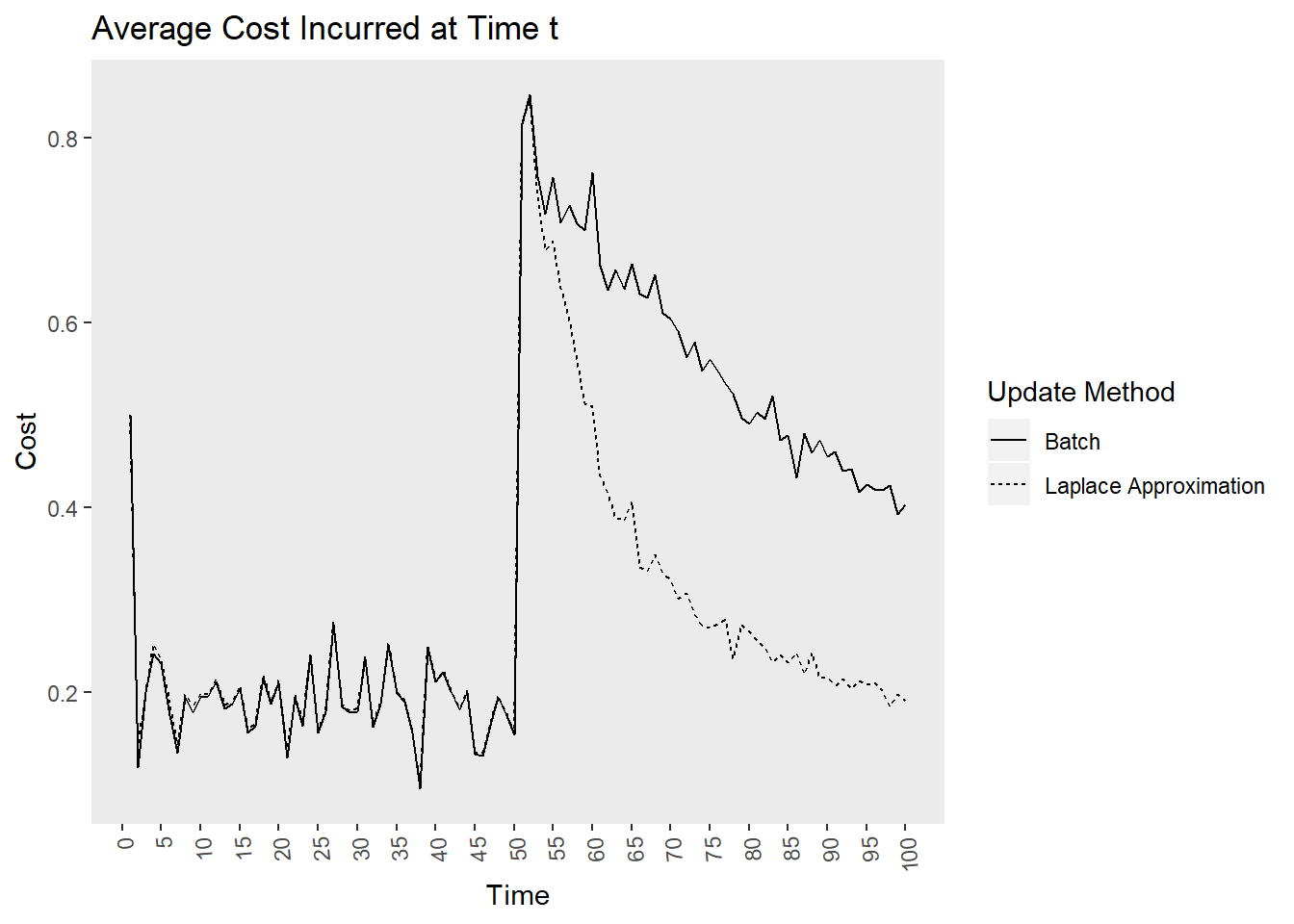
Conclusion
Bayesian modeling seems to offer several marked advantages. The incorporation of priors reduces data storage requirements while increasing the models flexibility as an adaptive learner. When the process that is trying to be modeled is stationary, both Bayesian and frequentist models seem to perform pretty equally. However, approximations to the posterior remedy the downsides of Bayesian modeling (speed and availability) in the case of logistic regression. While hardcore frequentists may take offense, I see no reason why Bayesian modeling should not be adopted!
Readings on Bayesian Methods and Logistic Regression
- Chapters 1 and 11 from Bayesian Data Analysis by Gelman and colleagues do a great job covering Bayesian perspectives and MCMC.
- Chapter 8 from Kevin Murphy’s Machine Learning: A Probabilistic Perspective provides a great overview of logistic regression and Bayesian approaches.
- Chapter 4 from Bishop’s Pattern Recognition and Machine Learning covers LaPlace approximations and logistic regression.